September Student post: Introduction to SQL

This is a quick-and-dirty introduction that will explain what SQL is, how it is used, and what some SQL queries look like in R using the dplyr package. SQL (sometimes pronounced “sequel”) stands for Structured Query Language. It is a programming language used to manipulate data in Relational Database Management Systems and it “is one of the most common languages for interacting with data” (source sqltutorial.org). SQL consists of three main languages under the same umbrella:

• data definition language - deals with database creation and modification
• data manipulation language - provides constructs to query and update data
• data control language - statements that deal with user authorization and security

Though SQL has a specific set of standards written by the American Standards Institute (ANSI), the user base constantly requires new features and capabilities. To accommodate this, there are a few different SQL “dialects” created by companies such as Oracle and Microsoft each with different syntaxes. In this tutorial, all SQL syntax used will be valid across all database systems.

Before going into SQL code, there are some important terms to know before creating a database. A primary key is a column or set of columns in a table whose value is unique for every record in the table. This can often be as simple as an integer ID or the combination of an ID and a date. A foreign key is a column in the table that refers to the primary key of another table. An example of this could be a situation where there is a table for purchases with a column for item number. The item number column is a foreign key that refers to the primary key item number of an items table with product information. For a more in-depth tutorial, I suggest reading through the Programiz tutorial.

Building a database in SQL

Building a database requires a schema. This shows the organization of the data as a blueprint of how the database is constructed. Below is an example of a simple relational database schema with seven tables: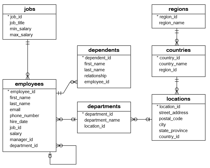

(image source)

The above schema is actually incomplete as only primary keys are identified (with an *) and we are left to assume that foreign keys have the same column name as the primary key it refers to. For example, job_id in the employees table is a foreign key for the job_id primary key in the jobs table. The “crows feet” notation connecting each table defines how many of each record there is for each relationship. They aren’t as important when using SQL, but they are necessary knowledge when one has to interact with a real database. I’ll explain the relationship between employees and jobs as an example. The connector on the jobs table signifies that every employee has one and only one job_id reference to a job in the jobs table. The connector on the employees table means every job_id may be associated with zero or more records (people) in the employees table.

Data Definition Language

In the industry, these commands are often restricted to be used by only the Database Management group. This is so that no random person in the company can edit the database and potentially destroy sensitive information. To show examples of database creation using SQL, I will create the jobs table. The following code chunk contains comments with more details:

-- The notation at the start of this line denotes a comment, everything after "--" will be ignored
-- All SQL commands must end in a semicolon ";"
-- Most SQL command words are in all caps, but this can depend on the system
-- First we have to create the database, this one will be called "HR"
CREATE DATABASE HR;

-- The CREATE TABLE command creates a table and takes the columns with data types as the argument
-- The basic syntax looks like this:
CREATE TABLE table_name (
  column1 datatype,
  column2 datatype,
  ...
);

-- Here is the full code to create the jobs table:
CREATE TABLE jobs (
    job_id INT (11) AUTO_INCREMENT PRIMARY KEY,
    job_title VARCHAR (35) NOT NULL,
    min_salary DECIMAL (8, 2) DEFAULT NULL,
    max_salary DECIMAL (8, 2) DEFAULT NULL
);

In the above code chunk, there were some new commands that may not look familiar. I’ll explain each column line-by-line.

• The job_id column will be integer data. The number in parentheses tells the database the maximum number of digits that a job_id can have, in this case it is 11. The AUTO_INCREMENT command is an automatic function that runs whenever a new job is added to the table. Finally, PRIMARY KEY tells us this is the primary key.
• The job_title column has a datatype called VARCHAR. This is a keyword meaning character data that is varying, essentially it is string data. The maximum length of a job_title is 35 characters, and the row cannot be empty. The NOT NULL command forces all records to have a job_title.
• The last two columns, min_salary and max_salary, are very similar. They both have decimal data type, with 8 digits before the decimal and 2 digits after. Also, they both have DEFAULT NULL commands meaning that they are not required values when adding a new job. Adding a new job without specifying salaries will make those attributes empty.

To denote a foreign key, the structure looks like this:

CREATE TABLE table_name (
  column1 datatype,
  column2 datatype,
  ...
  -- column3 is a primary key in another table
  FOREIGN KEY (column2) REFERENCES another_table_name (column3)
);

Additional commands are necessary to add to CREATE TABLE for when a table or record is deleted, but those are beyond the scope of this introduction. Other commands in the Data Definition language are shown below:

-- See how these commands are not enclosed in parentheses?
-- Little syntax differences like these can depend on the specific software being used
-- However, all SQL commands end with a semicolon ;

ALTER TABLE table_name
ADD new_column datatype
DROP old_column
RENAME TO NEW_TABLE_NAME;

DROP TABLE table_name;

-- The ALTER TABLE command can also change column names and data definitions with RENAME and MODIFY

Data Control Language

There are only two main commands in this language. They are GRANT and REVOKE. Only Database Administrator’s or owner’s of the database object can provide/remove privileges on a database object. The details of these commands are beyond the scope of this introduction, but their skeleton will be shown.

The syntax for the GRANT command is:

GRANT privilege_name 
ON database_name 
TO {user_name |PUBLIC |role_name} -- username or all users or users with role_name
[WITH GRANT OPTION]; -- optional

The syntax for the REVOKE command is:

REVOKE privilege_name 
ON database_name 
FROM {user_name |PUBLIC |role_name}; -- username or all users or users with role_name

Data Manipulation Language

To demonstrate examples, I will create a couple of toy datasets: one for employees and one for jobs. In these examples, I did not include a primary key for employees so we can assume the first and last name together are the primary key. The primary key of the jobs table is job_id and the employees table has a foreign key with the same name.

employees <- tibble(
  first_name = c("Curly", "Larry", "Moe", "Joe"),
  last_name = c("Morris", "Cambridge", "Wallace", "Frasier"),
  salary = c(10000.00, 10000.00, 12500.00, 13333.33),
  job_id = c(1, 2, 3, 4)
)
head(employees)

## # A tibble: 4 × 4
##   first_name last_name salary job_id
##   <chr>      <chr>      <dbl>  <dbl>
## 1 Curly      Morris    10000       1
## 2 Larry      Cambridge 10000       2
## 3 Moe        Wallace   12500       3
## 4 Joe        Frasier   13333.      4

jobs <- tibble(
  job_title = c("Janitor", "Maintenenace", "Electrical", "Manager"),
  job_id = c(1, 2, 3, 4)
)
head(jobs)

## # A tibble: 4 × 2
##   job_title    job_id
##   <chr>         <dbl>
## 1 Janitor           1
## 2 Maintenenace      2
## 3 Electrical        3
## 4 Manager           4

For this introduction, I’ll focus on the SELECT command to make queries to the database. However, there are other commands in the language such as INSERT, UPDATE, and DELETE. The basic format of a SQL query looks like this:

SELECT select_list
FROM table_name;

Using R, this command would look like:

select(data = table_name, column1, column2, ...)

The select list can be any number of comma-separated column names or an asterisk * to denote all columns in the table. When evaluating the SELECT statement, the database system evaluates the FROM clause first and then the SELECT clause. You can also do arithmetic in the SELECT clause, a couple of examples are below with their R translation and output:

SELECT first_name, last_name, salary, salary * 1.25
FROM employees;

employees %>% select(first_name, last_name, salary) %>%
  mutate(raise = salary * 1.25)

## # A tibble: 4 × 4
##   first_name last_name salary  raise
##   <chr>      <chr>      <dbl>  <dbl>
## 1 Curly      Morris    10000  12500 
## 2 Larry      Cambridge 10000  12500 
## 3 Moe        Wallace   12500  15625 
## 4 Joe        Frasier   13333. 16667.

SELECT AVG(salary), COUNT(DISTINCT(salary)), ROUND(salary, 0) -- round to 0 decimal places
FROM employees;

employees %>% transmute(avg_salary = mean(salary),
          count_distinct = n_distinct(salary), trunc_salary = floor(salary))

## # A tibble: 4 × 3
##   avg_salary count_distinct trunc_salary
##        <dbl>          <int>        <dbl>
## 1     11458.              3        10000
## 2     11458.              3        10000
## 3     11458.              3        12500
## 4     11458.              3        13333

SELECT MAX(salary), MIN(salary)
FROM employees;

employees %>% transmute(max_sal = max(salary), min_sal = min(salary))

## # A tibble: 4 × 2
##   max_sal min_sal
##     <dbl>   <dbl>
## 1  13333.   10000
## 2  13333.   10000
## 3  13333.   10000
## 4  13333.   10000

To get data from other tables and join it to this one, we use a JOIN clause. Using INNER JOIN, we can select the rows that have a record in both tables. SQL also supports LEFT JOIN and RIGHT JOIN. The format looks like this:

SELECT first_name, last_name, job_title
FROM employees
INNER JOIN jobs ON job_id = job_id;
-- the name before the equals sign is the primary key in the employees table

In R, it might look like this:

employees %>% select(first_name, last_name, job_id) %>%
  inner_join(jobs, by=c("job_id"="job_id"))

## # A tibble: 4 × 4
##   first_name last_name job_id job_title   
##   <chr>      <chr>      <dbl> <chr>       
## 1 Curly      Morris         1 Janitor     
## 2 Larry      Cambridge      2 Maintenenace
## 3 Moe        Wallace        3 Electrical  
## 4 Joe        Frasier        4 Manager

SQL queries can be powerful, and they can also get huge if you have to join multiple tables. This introduction does not go in depth, so to learn more you should do some research. If you know R, you will see some parallels between the dplyr package and SQL queries. In fact, R actually supports SQL to get data straight from central relational databases. In this introductory tutorial, databases were introduced, basic examples were given for each of the three SQL languages, and some queries were shown in the R programming language.

---

Joseph Shifman is a Computer Science major with a minor in Math. He is also in the Data Science Certificate program at CSU Chico. To see more projects he has worked on, check out his Github or his LinkedIn.